
Integrating optimisation strategies into an aquathermal energy system can lead to a significant reduction in energy costs. Two key variables play a central role in this equation: accurate predictions of energy consumption and generation, as well as the ability to adapt consumption and leverage buffer capacity.
Setting the scene: What do we mean by an optimised energy system?
Let’s consider an energy system that has solar panels, warm water buffers, aquathermal heat exchangers and 20 consumers using the system for heating and warm water supply.
Scenario 1: A baseline aquathermal energy system.
The system exclusively relies on local technical control loops to manage the heat pumps and water buffers. The system steadily heats the buffers until 40 degrees and then wait for demand. If the demand peaks at a moment without sun, the system will consume electricity from the grid to run the heat pumps.
Scenario 2: A smart aquathermal energy system.
The system relies on a software made to forecast consumption based on history and other variables. The system will pre-heat the buffers until 55 degrees using solar energy – thus, with minimal costs - ahead of the peak demand. . When peak demand occurs, the heat pump only needs to supply a very limited amount of energy because the buffer temperature is already close to 60 degrees.
Smart energy system: How do the technical software and the intelligent forecasting interact?
In a smart energy system (scenario 2), the technical and forecasting systems interact by continuously exchanging information, enabling the system to operate in an optimised manner. Running stand-alone, the technical system software maintains minimum and maximum temperatures and controls grid electricity consumption. It also signals errors and warnings in the system. Preferably, the system should not contain any further intelligence.
Meanwhile, the forecasting system sends hourly temperature targets to the technical system, which the heatpumps will take as new setpoints. Inversely, the technical system continuously sends sensor data to the forecasting system. Minimum data points are: buffer temperatures, heat consumption, power consumption of the heat pumps, warnings and errors. Communication between the two systems will normally use a REST-API or Modbus communication standards.
What is needed for a proper forecast?
The first step is to collect accurate and reliable data. This needs to be done in a well-documented manner, meaning that any error in the data collection should be signaled immediately.
An example of collected data items is the following:
- Historical energy consumption (electricity and gas)
- Weather forecast
- Number of consumers, current and expected
- Holidays
- Current external/internal air and water temperatures
- Current electricity/ gas consumption
- Current buffer capacity and temperatures
- Status/ capacity of heat pumps
- Electricity prices
- Solar panel capacity
Once the data is collected, a forecast can be generated for the next 24 hours, updated every hour to create a rolling forecast. Each hour, the expected heat demand is predicted based on weather conditions, the number of consumers, and the demand profile. In parallel, the hourly available energy is calculated based on grid capacity, other electricity consumers, and solar panel output forecasts..
The optimisation of the heat pumps can be performed using linear programming. A simple model is defined as follows:
Objective:
- Minimise grid costs
Parameters:
- Heat pump capacity: between 0 and 80 kW
- Buffer capacity: between 0 and 300 kWh, minimum is 6 kWh
- Heat pump COP: 3
Inputs:
- Heat demand per hour
- Available grid electricity per hour
- Available solar energy per hour
Using linear programming, an optimal solution can be calculated.
Tip: use Python with PuLP
As an illustration, a sample output is displayed below:
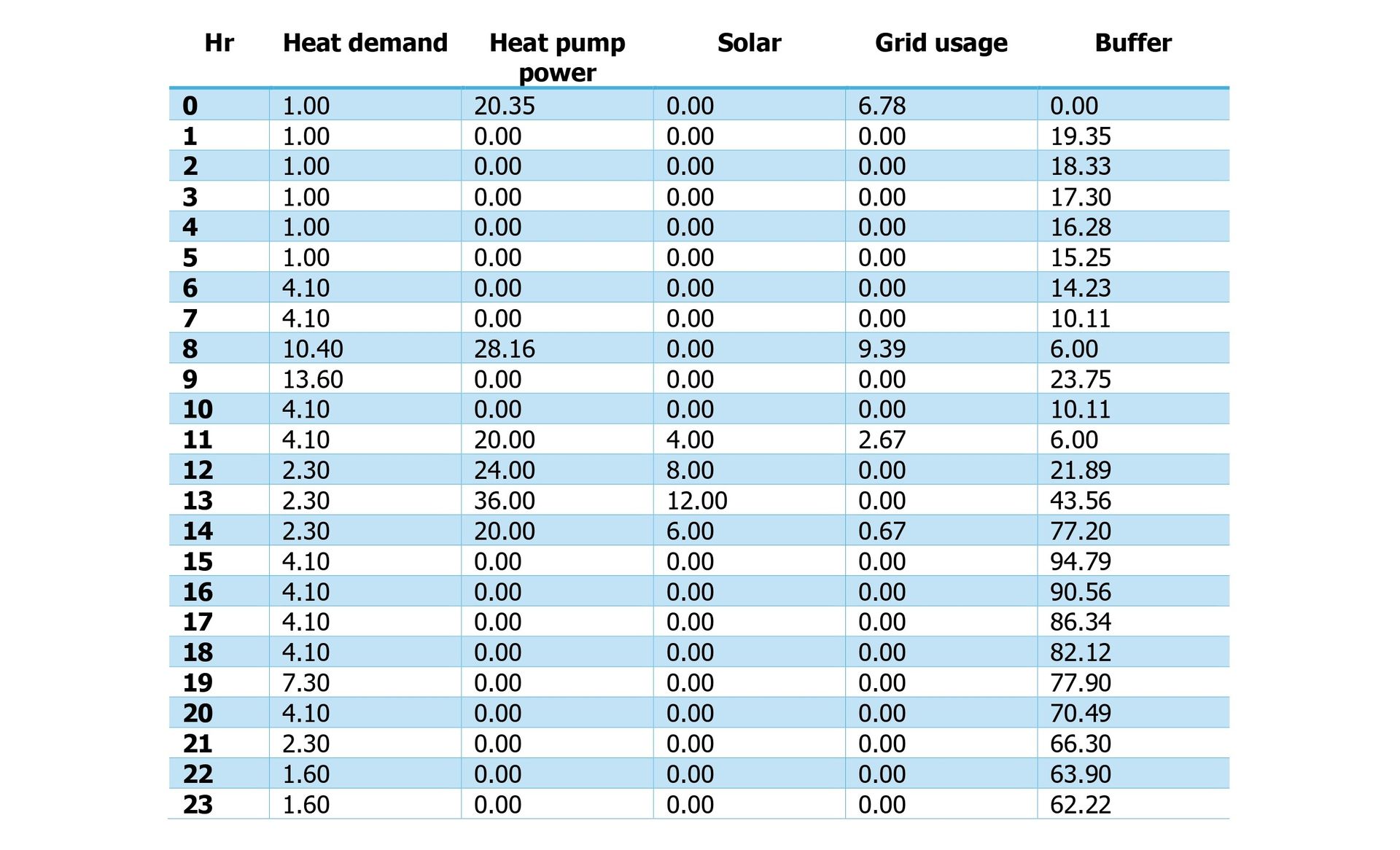
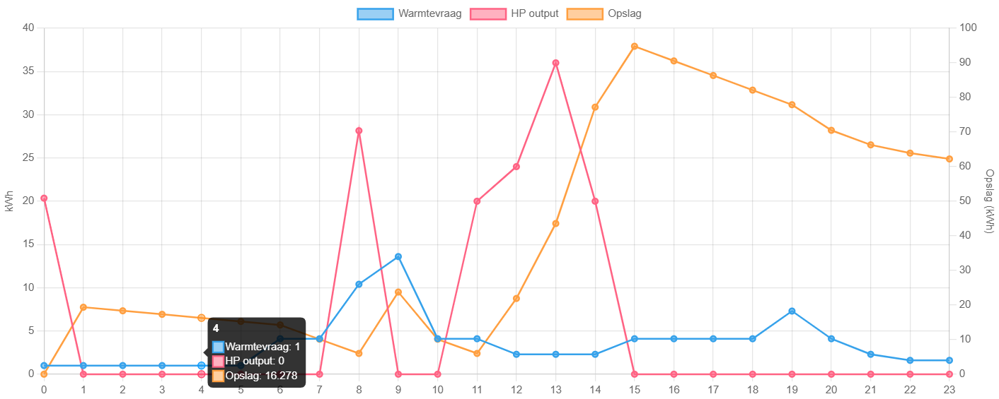
While the heat demand peaks in the morning and late afternoon, solar energy peaks at midday. The model uses solar power as much as possible and adds buffered energy as soon as solar becomes available. Grid power is used in advance to prepare for the morning peak in demand and to maintain the buffer above its defined minimum capacity.
The model can be further optimised by adding constraints for the heat pumps (e.g. minimum power, minimum running time), efficiency losses, heat loss (or gain) in the network and heat loss of the buffers.